The Batch Normalization layer of Keras is damaged

UPDATE: Sadly my Pull-Request to Keras that modified the behaviour of the Batch Normalization layer was not accepted. You may learn the main points right here. For these of you who’re courageous sufficient to mess with customized implementations, yow will discover the code in my department. I’d preserve it and merge it with the newest steady model of Keras (2.1.6, 2.2.2 and 2.2.4) for so long as I take advantage of it however no guarantees.

Most individuals who work in Deep Studying have both used or heard of Keras. For these of you who haven’t, it’s an ideal library that abstracts the underlying Deep Studying frameworks reminiscent of TensorFlow, Theano and CNTK and gives a high-level API for coaching ANNs. It’s straightforward to make use of, allows quick prototyping and has a pleasant lively group. I’ve been utilizing it closely and contributing to the challenge periodically for fairly a while and I positively suggest it to anybody who desires to work on Deep Studying.

Although Keras made my life simpler, fairly many instances I’ve been bitten by the odd conduct of the Batch Normalization layer. Its default conduct has modified over time, nonetheless it nonetheless causes issues to many customers and consequently there are a number of associated open points on Github. On this weblog submit, I’ll attempt to construct a case for why Keras’ BatchNormalization layer doesn’t play good with Switch Studying, I’ll present the code that fixes the issue and I’ll give examples with the outcomes of the patch.

On the subsections under, I present an introduction on how Switch Studying is utilized in Deep Studying, what’s the Batch Normalization layer, how learnining_phase works and the way Keras modified the BN conduct over time. In case you already know these, you possibly can safely bounce on to part 2.

1.1 Utilizing Switch Studying is essential for Deep Studying

One of many the explanation why Deep Studying was criticized previously is that it requires an excessive amount of information. This isn’t at all times true; there are a number of strategies to handle this limitation, considered one of which is Switch Studying.

Assume that you’re engaged on a Laptop Imaginative and prescient utility and also you wish to construct a classifier that distinguishes Cats from Canine. You don’t really want thousands and thousands of cat/canine photographs to coach the mannequin. As an alternative you should use a pre-trained classifier and fine-tune the highest convolutions with much less information. The thought behind it’s that for the reason that pre-trained mannequin was match on photographs, the underside convolutions can acknowledge options like traces, edges and different helpful patterns which means you should use its weights both nearly as good initialization values or partially retrain the community together with your information.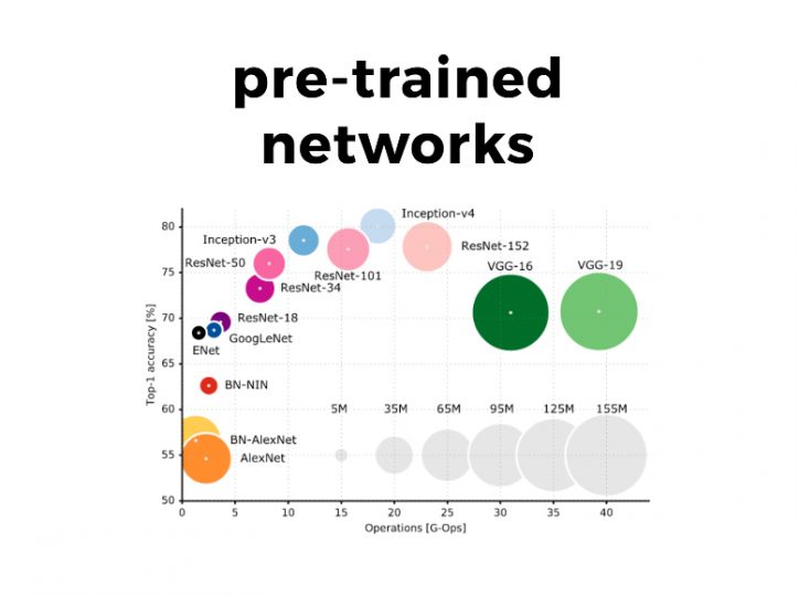

Keras comes with a number of pre-trained fashions and easy-to-use examples on fine-tune fashions. You may learn extra on the documentation.

1.2 What’s the Batch Normalization layer?

The Batch Normalization layer was launched in 2014 by Ioffe and Szegedy. It addresses the vanishing gradient drawback by standardizing the output of the earlier layer, it hastens the coaching by decreasing the variety of required iterations and it allows the coaching of deeper neural networks. Explaining precisely the way it works is past the scope of this submit however I strongly encourage you to learn the unique paper. An oversimplified rationalization is that it rescales the enter by subtracting its imply and by dividing with its customary deviation; it will possibly additionally study to undo the transformation if obligatory.

1.3 What’s the learning_phase in Keras?

Some layers function in a different way throughout coaching and inference mode. Essentially the most notable examples are the Batch Normalization and the Dropout layers. Within the case of BN, throughout coaching we use the imply and variance of the mini-batch to rescale the enter. However, throughout inference we use the shifting common and variance that was estimated throughout coaching.

Keras is aware of through which mode to run as a result of it has a built-in mechanism known as learning_phase. The educational section controls whether or not the community is on practice or check mode. If it’s not manually set by the consumer, throughout match() the community runs with learning_phase=1 (practice mode). Whereas producing predictions (for instance once we name the predict() & consider() strategies or on the validation step of the match()) the community runs with learning_phase=0 (check mode). Although it’s not advisable, the consumer can be in a position to statically change the learning_phase to a particular worth however this must occur earlier than any mannequin or tensor is added within the graph. If the learning_phase is about statically, Keras shall be locked to whichever mode the consumer chosen.

1.4 How did Keras implement Batch Normalization over time?

Keras has modified the conduct of Batch Normalization a number of instances however the latest important replace occurred in Keras 2.1.3. Earlier than v2.1.3 when the BN layer was frozen (trainable = False) it saved updating its batch statistics, one thing that triggered epic complications to its customers.

This was not only a bizarre coverage, it was truly fallacious. Think about {that a} BN layer exists between convolutions; if the layer is frozen no adjustments ought to occur to it. If we do replace partially its weights and the following layers are additionally frozen, they’ll by no means get the possibility to regulate to the updates of the mini-batch statistics resulting in increased error. Fortunately ranging from model 2.1.3, when a BN layer is frozen it not updates its statistics. However is that sufficient? Not in case you are utilizing Switch Studying.

Beneath I describe precisely what’s the drawback and I sketch out the technical implementation for fixing it. I additionally present a number of examples to indicate the results on mannequin’s accuracy earlier than and after the patch is utilized.

2.1 Technical description of the issue

The issue with the present implementation of Keras is that when a BN layer is frozen, it continues to make use of the mini-batch statistics throughout coaching. I consider a greater method when the BN is frozen is to make use of the shifting imply and variance that it discovered throughout coaching. Why? For a similar the explanation why the mini-batch statistics shouldn’t be up to date when the layer is frozen: it will possibly result in poor outcomes as a result of the following layers should not skilled correctly.

Assume you might be constructing a Laptop Imaginative and prescient mannequin however you don’t have sufficient information, so that you resolve to make use of one of many pre-trained CNNs of Keras and fine-tune it. Sadly, by doing so that you get no ensures that the imply and variance of your new dataset contained in the BN layers shall be much like those of the unique dataset. Do not forget that in the meanwhile, throughout coaching your community will at all times use the mini-batch statistics both the BN layer is frozen or not; additionally throughout inference you’ll use the beforehand discovered statistics of the frozen BN layers. Because of this, should you fine-tune the highest layers, their weights shall be adjusted to the imply/variance of the new dataset. However, throughout inference they’ll obtain information that are scaled in a different way as a result of the imply/variance of the unique dataset shall be used.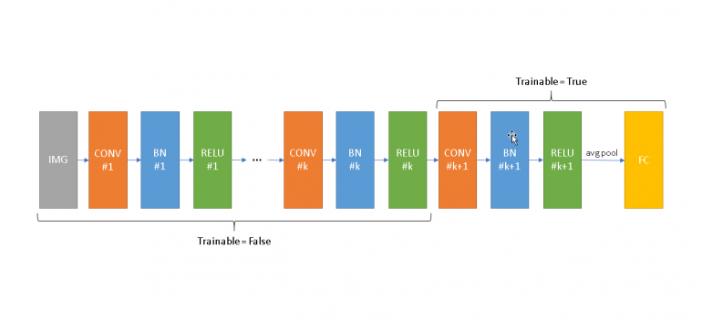

Above I present a simplistic (and unrealistic) structure for demonstration functions. Let’s assume that we fine-tune the mannequin from Convolution okay+1 up till the highest of the community (proper aspect) and we maintain frozen the underside (left aspect). Throughout coaching all BN layers from 1 to okay will use the imply/variance of your coaching information. It will have adverse results on the frozen ReLUs if the imply and variance on every BN should not near those discovered throughout pre-training. It can additionally trigger the remainder of the community (from CONV okay+1 and later) to be skilled with inputs which have completely different scales evaluating to what’s going to obtain throughout inference. Throughout coaching your community can adapt to those adjustments, nonetheless the second you turn to prediction-mode, Keras will use completely different standardization statistics, one thing that can swift the distribution of the inputs of the following layers resulting in poor outcomes.

2.2 How will you detect in case you are affected?

One approach to detect it’s to set statically the educational section of Keras to 1 (practice mode) and to 0 (check mode) and consider your mannequin in every case. If there’s important distinction in accuracy on the identical dataset, you might be being affected by the issue. It’s price declaring that, as a result of manner the learning_phase mechanism is carried out in Keras, it’s usually not suggested to mess with it. Modifications on the learning_phase could have no impact on fashions which are already compiled and used; as you possibly can see on the examples on the following subsections, one of the simplest ways to do that is to start out with a clear session and alter the learning_phase earlier than any tensor is outlined within the graph.

One other approach to detect the issue whereas working with binary classifiers is to examine the accuracy and the AUC. If the accuracy is near 50% however the AUC is near 1 (and in addition you observe variations between practice/check mode on the identical dataset), it might be that the possibilities are out-of-scale due the BN statistics. Equally, for regression you should use MSE and Spearman’s correlation to detect it.

2.3 How can we repair it?

I consider that the issue may be mounted if the frozen BN layers are literally simply that: completely locked in check mode. Implementation-wise, the trainable flag must be a part of the computational graph and the conduct of the BN must rely not solely on the learning_phase but additionally on the worth of the trainable property. You’ll find the main points of my implementation on Github.

By making use of the above repair, when a BN layer is frozen it would not use the mini-batch statistics however as a substitute use those discovered throughout coaching. Because of this, there shall be no discrepancy between coaching and check modes which results in elevated accuracy. Clearly when the BN layer will not be frozen, it would proceed utilizing the mini-batch statistics throughout coaching.

2.4 Assessing the results of the patch

Although I wrote the above implementation just lately, the thought behind it’s closely examined on real-world issues utilizing varied workarounds which have the identical impact. For instance, the discrepancy between coaching and testing modes and may be averted by splitting the community in two components (frozen and unfrozen) and performing cached coaching (passing information via the frozen mannequin as soon as after which utilizing them to coach the unfrozen community). However, as a result of the “belief me I’ve achieved this earlier than” usually bears no weight, under I present a number of examples that present the results of the brand new implementation in follow.

Listed here are a number of essential factors in regards to the experiment:

1. I’ll use a tiny quantity of information to deliberately overfit the mannequin and I’ll practice & validate the mannequin on the identical dataset. By doing so, I count on close to excellent accuracy and similar efficiency on the practice/validation dataset.
2. If throughout validation I get considerably decrease accuracy on the identical dataset, I’ll have a transparent indication that the present BN coverage impacts negatively the efficiency of the mannequin throughout inference.
3. Any preprocessing will happen exterior of Mills. That is achieved to work round a bug that was launched in v2.1.5 (at present mounted on upcoming v2.1.6 and newest grasp).
4. We are going to pressure Keras to make use of completely different studying phases throughout analysis. If we spot variations between the reported accuracy we are going to know we’re affected by the present BN coverage.

The code for the experiment is proven under:

import numpy as np
from keras.datasets import cifar10
from scipy.misc import imresize

from keras.preprocessing.picture import ImageDataGenerator
from keras.functions.resnet50 import ResNet50, preprocess_input
from keras.fashions import Mannequin, load_model
from keras.layers import Dense, Flatten
from keras import backend as Ok


seed = 42
epochs = 10
records_per_class = 100

# We take solely 2 lessons from CIFAR10 and a really small pattern to deliberately overfit the mannequin.
# We may also use the identical information for practice/check and count on that Keras will give the identical accuracy.
(x, y), _ = cifar10.load_data()

def filter_resize(class):
   # We do the preprocessing right here as a substitute within the Generator to get round a bug on Keras 2.1.5.
   return [preprocess_input(imresize(img, (224,224)).astype('float')) for img in x[y.flatten()==category][:records_per_class]]

x = np.stack(filter_resize(3)+filter_resize(5))
records_per_class = x.form[0] // 2
y = np.array([[1,0]]*records_per_class + [[0,1]]*records_per_class)


# We are going to use a pre-trained mannequin and finetune the highest layers.
np.random.seed(seed)
base_model = ResNet50(weights="imagenet", include_top=False, input_shape=(224, 224, 3))
l = Flatten()(base_model.output)
predictions = Dense(2, activation='softmax')(l)
mannequin = Mannequin(inputs=base_model.enter, outputs=predictions)

for layer in mannequin.layers[:140]:
   layer.trainable = False

for layer in mannequin.layers[140:]:
   layer.trainable = True

mannequin.compile(optimizer="sgd", loss="categorical_crossentropy", metrics=['accuracy'])
mannequin.fit_generator(ImageDataGenerator().move(x, y, seed=42), epochs=epochs, validation_data=ImageDataGenerator().move(x, y, seed=42))

# Retailer the mannequin on disk
mannequin.save('tmp.h5')


# In each check we are going to clear the session and reload the mannequin to pressure Learning_Phase values to vary.
print('DYNAMIC LEARNING_PHASE')
Ok.clear_session()
mannequin = load_model('tmp.h5')
# This accuracy ought to match precisely the one of many validation set on the final iteration.
print(mannequin.evaluate_generator(ImageDataGenerator().move(x, y, seed=42)))


print('STATIC LEARNING_PHASE = 0')
Ok.clear_session()
Ok.set_learning_phase(0)
mannequin = load_model('tmp.h5')
# Once more the accuracy ought to match the above.
print(mannequin.evaluate_generator(ImageDataGenerator().move(x, y, seed=42)))


print('STATIC LEARNING_PHASE = 1')
Ok.clear_session()
Ok.set_learning_phase(1)
mannequin = load_model('tmp.h5')
# The accuracy shall be near the one of many coaching set on the final iteration.
print(mannequin.evaluate_generator(ImageDataGenerator().move(x, y, seed=42)))

Let’s examine the outcomes on Keras v2.1.5:

Epoch 1/10
1/7 [===>..........................] - ETA: 25s - loss: 0.8751 - acc: 0.5312
2/7 [=======>......................] - ETA: 11s - loss: 0.8594 - acc: 0.4531
3/7 [===========>..................] - ETA: 7s - loss: 0.8398 - acc: 0.4688 
4/7 [================>.............] - ETA: 4s - loss: 0.8467 - acc: 0.4844
5/7 [====================>.........] - ETA: 2s - loss: 0.7904 - acc: 0.5437
6/7 [========================>.....] - ETA: 1s - loss: 0.7593 - acc: 0.5625
7/7 [==============================] - 12s 2s/step - loss: 0.7536 - acc: 0.5744 - val_loss: 0.6526 - val_acc: 0.6650

Epoch 2/10
1/7 [===>..........................] - ETA: 4s - loss: 0.3881 - acc: 0.8125
2/7 [=======>......................] - ETA: 3s - loss: 0.3945 - acc: 0.7812
3/7 [===========>..................] - ETA: 2s - loss: 0.3956 - acc: 0.8229
4/7 [================>.............] - ETA: 1s - loss: 0.4223 - acc: 0.8047
5/7 [====================>.........] - ETA: 1s - loss: 0.4483 - acc: 0.7812
6/7 [========================>.....] - ETA: 0s - loss: 0.4325 - acc: 0.7917
7/7 [==============================] - 8s 1s/step - loss: 0.4095 - acc: 0.8089 - val_loss: 0.4722 - val_acc: 0.7700

Epoch 3/10
1/7 [===>..........................] - ETA: 4s - loss: 0.2246 - acc: 0.9375
2/7 [=======>......................] - ETA: 3s - loss: 0.2167 - acc: 0.9375
3/7 [===========>..................] - ETA: 2s - loss: 0.2260 - acc: 0.9479
4/7 [================>.............] - ETA: 2s - loss: 0.2179 - acc: 0.9375
5/7 [====================>.........] - ETA: 1s - loss: 0.2356 - acc: 0.9313
6/7 [========================>.....] - ETA: 0s - loss: 0.2392 - acc: 0.9427
7/7 [==============================] - 8s 1s/step - loss: 0.2288 - acc: 0.9456 - val_loss: 0.4282 - val_acc: 0.7800

Epoch 4/10
1/7 [===>..........................] - ETA: 4s - loss: 0.2183 - acc: 0.9688
2/7 [=======>......................] - ETA: 3s - loss: 0.1899 - acc: 0.9844
3/7 [===========>..................] - ETA: 2s - loss: 0.1887 - acc: 0.9792
4/7 [================>.............] - ETA: 1s - loss: 0.1995 - acc: 0.9531
5/7 [====================>.........] - ETA: 1s - loss: 0.1932 - acc: 0.9625
6/7 [========================>.....] - ETA: 0s - loss: 0.1819 - acc: 0.9688
7/7 [==============================] - 8s 1s/step - loss: 0.1743 - acc: 0.9747 - val_loss: 0.3778 - val_acc: 0.8400

Epoch 5/10
1/7 [===>..........................] - ETA: 3s - loss: 0.0973 - acc: 1.0000
2/7 [=======>......................] - ETA: 3s - loss: 0.0828 - acc: 1.0000
3/7 [===========>..................] - ETA: 2s - loss: 0.0851 - acc: 1.0000
4/7 [================>.............] - ETA: 1s - loss: 0.0897 - acc: 1.0000
5/7 [====================>.........] - ETA: 1s - loss: 0.0928 - acc: 1.0000
6/7 [========================>.....] - ETA: 0s - loss: 0.0936 - acc: 1.0000
7/7 [==============================] - 8s 1s/step - loss: 0.1337 - acc: 0.9838 - val_loss: 0.3916 - val_acc: 0.8100

Epoch 6/10
1/7 [===>..........................] - ETA: 4s - loss: 0.0747 - acc: 1.0000
2/7 [=======>......................] - ETA: 3s - loss: 0.0852 - acc: 1.0000
3/7 [===========>..................] - ETA: 2s - loss: 0.0812 - acc: 1.0000
4/7 [================>.............] - ETA: 1s - loss: 0.0831 - acc: 1.0000
5/7 [====================>.........] - ETA: 1s - loss: 0.0779 - acc: 1.0000
6/7 [========================>.....] - ETA: 0s - loss: 0.0766 - acc: 1.0000
7/7 [==============================] - 8s 1s/step - loss: 0.0813 - acc: 1.0000 - val_loss: 0.3637 - val_acc: 0.8550

Epoch 7/10
1/7 [===>..........................] - ETA: 1s - loss: 0.2478 - acc: 0.8750
2/7 [=======>......................] - ETA: 2s - loss: 0.1966 - acc: 0.9375
3/7 [===========>..................] - ETA: 2s - loss: 0.1528 - acc: 0.9583
4/7 [================>.............] - ETA: 1s - loss: 0.1300 - acc: 0.9688
5/7 [====================>.........] - ETA: 1s - loss: 0.1193 - acc: 0.9750
6/7 [========================>.....] - ETA: 0s - loss: 0.1196 - acc: 0.9792
7/7 [==============================] - 8s 1s/step - loss: 0.1084 - acc: 0.9838 - val_loss: 0.3546 - val_acc: 0.8600

Epoch 8/10
1/7 [===>..........................] - ETA: 4s - loss: 0.0539 - acc: 1.0000
2/7 [=======>......................] - ETA: 2s - loss: 0.0900 - acc: 1.0000
3/7 [===========>..................] - ETA: 2s - loss: 0.0815 - acc: 1.0000
4/7 [================>.............] - ETA: 1s - loss: 0.0740 - acc: 1.0000
5/7 [====================>.........] - ETA: 1s - loss: 0.0700 - acc: 1.0000
6/7 [========================>.....] - ETA: 0s - loss: 0.0701 - acc: 1.0000
7/7 [==============================] - 8s 1s/step - loss: 0.0695 - acc: 1.0000 - val_loss: 0.3269 - val_acc: 0.8600

Epoch 9/10
1/7 [===>..........................] - ETA: 4s - loss: 0.0306 - acc: 1.0000
2/7 [=======>......................] - ETA: 3s - loss: 0.0377 - acc: 1.0000
3/7 [===========>..................] - ETA: 2s - loss: 0.0898 - acc: 0.9583
4/7 [================>.............] - ETA: 1s - loss: 0.0773 - acc: 0.9688
5/7 [====================>.........] - ETA: 1s - loss: 0.0742 - acc: 0.9750
6/7 [========================>.....] - ETA: 0s - loss: 0.0708 - acc: 0.9792
7/7 [==============================] - 8s 1s/step - loss: 0.0659 - acc: 0.9838 - val_loss: 0.3604 - val_acc: 0.8600

Epoch 10/10
1/7 [===>..........................] - ETA: 3s - loss: 0.0354 - acc: 1.0000
2/7 [=======>......................] - ETA: 3s - loss: 0.0381 - acc: 1.0000
3/7 [===========>..................] - ETA: 2s - loss: 0.0354 - acc: 1.0000
4/7 [================>.............] - ETA: 1s - loss: 0.0828 - acc: 0.9688
5/7 [====================>.........] - ETA: 1s - loss: 0.0791 - acc: 0.9750
6/7 [========================>.....] - ETA: 0s - loss: 0.0794 - acc: 0.9792
7/7 [==============================] - 8s 1s/step - loss: 0.0704 - acc: 0.9838 - val_loss: 0.3615 - val_acc: 0.8600

DYNAMIC LEARNING_PHASE
[0.3614931714534759, 0.86]

STATIC LEARNING_PHASE = 0
[0.3614931714534759, 0.86]

STATIC LEARNING_PHASE = 1
[0.025861846953630446, 1.0]

As we will see above, throughout coaching the mannequin learns very effectively the information and achieves on the coaching set near-perfect accuracy. Nonetheless on the finish of every iteration, whereas evaluating the mannequin on the identical dataset, we get important variations in loss and accuracy. Notice that we shouldn’t be getting this; now we have overfitted deliberately the mannequin on the precise dataset and the coaching/validation datasets are similar.

After the coaching is accomplished we consider the mannequin utilizing 3 completely different learning_phase configurations: Dynamic, Static = 0 (check mode) and Static = 1 (coaching mode). As we will see the primary two configurations will present similar outcomes when it comes to loss and accuracy and their worth matches the reported accuracy of the mannequin on the validation set within the final iteration. However, as soon as we swap to coaching mode, we observe a large discrepancy (enchancment).  Why it that? As we mentioned earlier, the weights of the community are tuned anticipating to obtain information scaled with the imply/variance of the coaching information. Sadly, these statistics are completely different from those saved within the BN layers. For the reason that BN layers had been frozen, these statistics had been by no means up to date. This discrepancy between the values of the BN statistics results in the deterioration of the accuracy throughout inference.

Let’s see what occurs as soon as we apply the patch:

Epoch 1/10
1/7 [===>..........................] - ETA: 26s - loss: 0.9992 - acc: 0.4375
2/7 [=======>......................] - ETA: 12s - loss: 1.0534 - acc: 0.4375
3/7 [===========>..................] - ETA: 7s - loss: 1.0592 - acc: 0.4479 
4/7 [================>.............] - ETA: 4s - loss: 0.9618 - acc: 0.5000
5/7 [====================>.........] - ETA: 2s - loss: 0.8933 - acc: 0.5250
6/7 [========================>.....] - ETA: 1s - loss: 0.8638 - acc: 0.5417
7/7 [==============================] - 13s 2s/step - loss: 0.8357 - acc: 0.5570 - val_loss: 0.2414 - val_acc: 0.9450

Epoch 2/10
1/7 [===>..........................] - ETA: 4s - loss: 0.2331 - acc: 0.9688
2/7 [=======>......................] - ETA: 2s - loss: 0.3308 - acc: 0.8594
3/7 [===========>..................] - ETA: 2s - loss: 0.3986 - acc: 0.8125
4/7 [================>.............] - ETA: 1s - loss: 0.3721 - acc: 0.8281
5/7 [====================>.........] - ETA: 1s - loss: 0.3449 - acc: 0.8438
6/7 [========================>.....] - ETA: 0s - loss: 0.3168 - acc: 0.8646
7/7 [==============================] - 9s 1s/step - loss: 0.3165 - acc: 0.8633 - val_loss: 0.1167 - val_acc: 0.9950

Epoch 3/10
1/7 [===>..........................] - ETA: 1s - loss: 0.2457 - acc: 1.0000
2/7 [=======>......................] - ETA: 2s - loss: 0.2592 - acc: 0.9688
3/7 [===========>..................] - ETA: 2s - loss: 0.2173 - acc: 0.9688
4/7 [================>.............] - ETA: 1s - loss: 0.2122 - acc: 0.9688
5/7 [====================>.........] - ETA: 1s - loss: 0.2003 - acc: 0.9688
6/7 [========================>.....] - ETA: 0s - loss: 0.1896 - acc: 0.9740
7/7 [==============================] - 9s 1s/step - loss: 0.1835 - acc: 0.9773 - val_loss: 0.0678 - val_acc: 1.0000

Epoch 4/10
1/7 [===>..........................] - ETA: 1s - loss: 0.2051 - acc: 1.0000
2/7 [=======>......................] - ETA: 2s - loss: 0.1652 - acc: 0.9844
3/7 [===========>..................] - ETA: 2s - loss: 0.1423 - acc: 0.9896
4/7 [================>.............] - ETA: 1s - loss: 0.1289 - acc: 0.9922
5/7 [====================>.........] - ETA: 1s - loss: 0.1225 - acc: 0.9938
6/7 [========================>.....] - ETA: 0s - loss: 0.1149 - acc: 0.9948
7/7 [==============================] - 9s 1s/step - loss: 0.1060 - acc: 0.9955 - val_loss: 0.0455 - val_acc: 1.0000

Epoch 5/10
1/7 [===>..........................] - ETA: 4s - loss: 0.0769 - acc: 1.0000
2/7 [=======>......................] - ETA: 2s - loss: 0.0846 - acc: 1.0000
3/7 [===========>..................] - ETA: 2s - loss: 0.0797 - acc: 1.0000
4/7 [================>.............] - ETA: 1s - loss: 0.0736 - acc: 1.0000
5/7 [====================>.........] - ETA: 1s - loss: 0.0914 - acc: 1.0000
6/7 [========================>.....] - ETA: 0s - loss: 0.0858 - acc: 1.0000
7/7 [==============================] - 9s 1s/step - loss: 0.0808 - acc: 1.0000 - val_loss: 0.0346 - val_acc: 1.0000

Epoch 6/10
1/7 [===>..........................] - ETA: 1s - loss: 0.1267 - acc: 1.0000
2/7 [=======>......................] - ETA: 2s - loss: 0.1039 - acc: 1.0000
3/7 [===========>..................] - ETA: 2s - loss: 0.0893 - acc: 1.0000
4/7 [================>.............] - ETA: 1s - loss: 0.0780 - acc: 1.0000
5/7 [====================>.........] - ETA: 1s - loss: 0.0758 - acc: 1.0000
6/7 [========================>.....] - ETA: 0s - loss: 0.0789 - acc: 1.0000
7/7 [==============================] - 9s 1s/step - loss: 0.0738 - acc: 1.0000 - val_loss: 0.0248 - val_acc: 1.0000

Epoch 7/10
1/7 [===>..........................] - ETA: 4s - loss: 0.0344 - acc: 1.0000
2/7 [=======>......................] - ETA: 3s - loss: 0.0385 - acc: 1.0000
3/7 [===========>..................] - ETA: 3s - loss: 0.0467 - acc: 1.0000
4/7 [================>.............] - ETA: 1s - loss: 0.0445 - acc: 1.0000
5/7 [====================>.........] - ETA: 1s - loss: 0.0446 - acc: 1.0000
6/7 [========================>.....] - ETA: 0s - loss: 0.0429 - acc: 1.0000
7/7 [==============================] - 9s 1s/step - loss: 0.0421 - acc: 1.0000 - val_loss: 0.0202 - val_acc: 1.0000

Epoch 8/10
1/7 [===>..........................] - ETA: 4s - loss: 0.0319 - acc: 1.0000
2/7 [=======>......................] - ETA: 3s - loss: 0.0300 - acc: 1.0000
3/7 [===========>..................] - ETA: 3s - loss: 0.0320 - acc: 1.0000
4/7 [================>.............] - ETA: 2s - loss: 0.0307 - acc: 1.0000
5/7 [====================>.........] - ETA: 1s - loss: 0.0303 - acc: 1.0000
6/7 [========================>.....] - ETA: 0s - loss: 0.0291 - acc: 1.0000
7/7 [==============================] - 9s 1s/step - loss: 0.0358 - acc: 1.0000 - val_loss: 0.0167 - val_acc: 1.0000

Epoch 9/10
1/7 [===>..........................] - ETA: 4s - loss: 0.0246 - acc: 1.0000
2/7 [=======>......................] - ETA: 3s - loss: 0.0255 - acc: 1.0000
3/7 [===========>..................] - ETA: 3s - loss: 0.0258 - acc: 1.0000
4/7 [================>.............] - ETA: 2s - loss: 0.0250 - acc: 1.0000
5/7 [====================>.........] - ETA: 1s - loss: 0.0252 - acc: 1.0000
6/7 [========================>.....] - ETA: 0s - loss: 0.0260 - acc: 1.0000
7/7 [==============================] - 9s 1s/step - loss: 0.0327 - acc: 1.0000 - val_loss: 0.0143 - val_acc: 1.0000

Epoch 10/10
1/7 [===>..........................] - ETA: 4s - loss: 0.0251 - acc: 1.0000
2/7 [=======>......................] - ETA: 2s - loss: 0.0228 - acc: 1.0000
3/7 [===========>..................] - ETA: 2s - loss: 0.0217 - acc: 1.0000
4/7 [================>.............] - ETA: 1s - loss: 0.0249 - acc: 1.0000
5/7 [====================>.........] - ETA: 1s - loss: 0.0244 - acc: 1.0000
6/7 [========================>.....] - ETA: 0s - loss: 0.0239 - acc: 1.0000
7/7 [==============================] - 9s 1s/step - loss: 0.0290 - acc: 1.0000 - val_loss: 0.0127 - val_acc: 1.0000

DYNAMIC LEARNING_PHASE
[0.012697912137955427, 1.0]

STATIC LEARNING_PHASE = 0
[0.012697912137955427, 1.0]

STATIC LEARNING_PHASE = 1
[0.01744014158844948, 1.0]

Initially, we observe that the community converges considerably sooner and achieves excellent accuracy. We additionally see that there isn’t a longer a discrepancy when it comes to accuracy once we swap between completely different learning_phase values.

2.5 How does the patch carry out on an actual dataset?

So how does the patch carry out on a extra sensible experiment? Let’s use Keras’ pre-trained ResNet50 (initially match on imagenet), take away the highest classification layer and fine-tune it with and with out the patch and examine the outcomes. For information, we are going to use CIFAR10 (the usual practice/check break up offered by Keras) and we are going to resize the photographs to 224×224 to make them suitable with the ResNet50’s enter measurement.

We are going to do 10 epochs to coach the highest classification layer utilizing RSMprop after which we are going to do one other 5 to fine-tune the whole lot after the 139th layer utilizing SGD(lr=1e-4, momentum=0.9). With out the patch our mannequin achieves an accuracy of 87.44%. Utilizing the patch, we get an accuracy of 92.36%, nearly 5 factors increased.

2.6 Ought to we apply the identical repair to different layers reminiscent of Dropout?

Batch Normalization will not be the one layer that operates in a different way between practice and check modes. Dropout and its variants even have the identical impact. Ought to we apply the identical coverage to all these layers? I consider not (although I’d love to listen to your ideas on this). The reason being that Dropout is used to keep away from overfitting, thus locking it completely to prediction mode throughout coaching would defeat its objective. What do you assume?

I strongly consider that this discrepancy have to be solved in Keras. I’ve seen much more profound results (from 100% right down to 50% accuracy) in real-world functions brought on by this drawback. I plan to ship already despatched a PR to Keras with the repair and hopefully will probably be accepted.

In case you favored this blogpost, please take a second to share it on Fb or Twitter. 🙂