TF-IDF vs. Embeddings: From Key phrases to Semantic Search

---

---

TF-IDF vs. Embeddings: From Key phrases to Semantic Search

On this tutorial, you’ll study what vector databases and embeddings actually are, why they matter for contemporary AI programs, and the way they allow semantic search and retrieval-augmented technology (RAG). You’ll begin from textual content embeddings, see how they map which means to geometry, and at last question them for similarity search — all with hands-on code.

This lesson is the first of a 3-part sequence on Retrieval Augmented Technology:

1. TF-IDF vs. Embeddings: From Key phrases to Semantic Search (this tutorial)
2. Lesson 2
3. Lesson 3

To learn to construct your personal semantic search basis from scratch, simply hold studying.

---

Collection Preamble: From Textual content to RAG

Earlier than we begin turning textual content into numbers, let’s zoom out and see the larger image.

This 3-part sequence is your step-by-step journey from uncooked textual content paperwork to a working Retrieval-Augmented Technology (RAG) pipeline — the identical structure behind instruments akin to ChatGPT’s shopping mode, Bing Copilot, and inner enterprise copilots.

By the tip, you’ll not solely perceive how semantic search and retrieval work but in addition have a reproducible, modular codebase that mirrors production-ready RAG programs.

---

What You’ll Construct Throughout the Collection

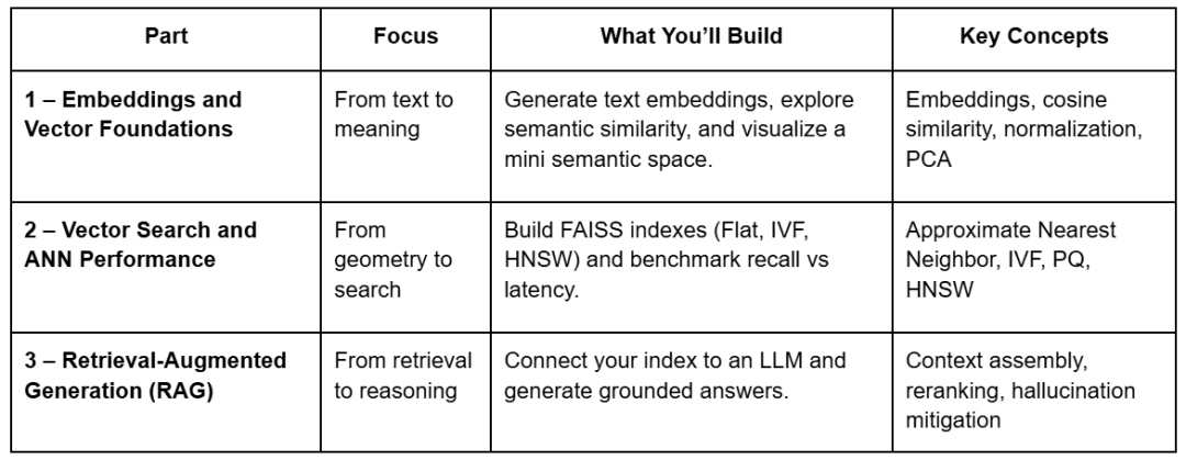
Every lesson builds on the final, utilizing the identical shared repository. You’ll see how a single set of embeddings evolves from a geometrical curiosity right into a working retrieval system with reasoning skills.

---

Challenge Construction

Earlier than writing code, let’s take a look at how the mission is organized.

All 3 classes share a single construction, so you’ll be able to reuse embeddings, indexes, and prompts throughout elements.

Beneath is the complete format — the recordsdata marked with Half 1 are those you’ll really contact on this lesson:

vector-rag-series/
├── 01_intro_to_embeddings.py          # Half 1 – generate & visualize embeddings
├── 02_vector_search_ann.py            # Half 2 – construct FAISS indexes & run ANN search
├── 03_rag_pipeline.py                 # Half 3 – join vector search to an LLM
│
├── pyimagesearch/
│   ├── __init__.py
│   ├── config.py                      # Paths, constants, mannequin title, immediate templates
│   ├── embeddings_utils.py            # Load corpus, generate & save embeddings
│   ├── vector_search_utils.py         # ANN utilities (Flat, IVF, HNSW)
│   └── rag_utils.py                   # Immediate builder & retrieval logic
│
├── information/
│   ├── enter/                         # Corpus textual content + metadata
│   ├── output/                        # Cached embeddings & PCA projection
│   ├── indexes/                       # FAISS indexes (used later)
│   └── figures/                       # Generated visualizations
│
├── scripts/
│   └── list_indexes.py                # Helper for index inspection (later)
│
├── atmosphere.yml                    # Conda atmosphere setup
├── necessities.txt                   # Dependencies
└── README.md                          # Collection overview & utilization information

In Lesson 1, we’ll concentrate on:

• config.py: centralized configuration and file paths
• embeddings_utils.py: core logic to load, embed, and save information
• 01_intro_to_embeddings.py: driver script orchestrating all the pieces

These elements type the spine of your semantic layer — all the pieces else (indexes, retrieval, and RAG logic) builds on high of this.

---

Why Begin with Embeddings

The whole lot begins with which means. Earlier than a pc can retrieve or cause about textual content, it should first signify what that textual content means.

Embeddings make this doable — they translate human language into numerical type, capturing delicate semantic relationships that key phrase matching can not.

On this 1st put up, you’ll:

• Generate textual content embeddings utilizing a transformer mannequin (sentence-transformers/all-MiniLM-L6-v2)
• Measure how related sentences are in which means utilizing cosine similarity
• Visualize how associated concepts naturally cluster in 2D area
• Persist your embeddings for quick retrieval in later classes

This basis will energy the ANN indexes in Half 2 and the complete RAG pipeline in Half 3.

With the roadmap and construction in place, let’s start our journey by understanding why conventional key phrase search falls brief — and the way embeddings remedy it.

---

The Drawback with Key phrase Search

Earlier than we discuss vector databases, let’s revisit the sort of search that dominated the net for many years: keyword-based retrieval.

Most classical programs (e.g., TF-IDF or BM25) deal with textual content as a bag of phrases. They depend how typically phrases seem, alter for rarity, and assume overlap = relevance.

That works… till it doesn’t.

---

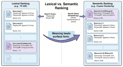
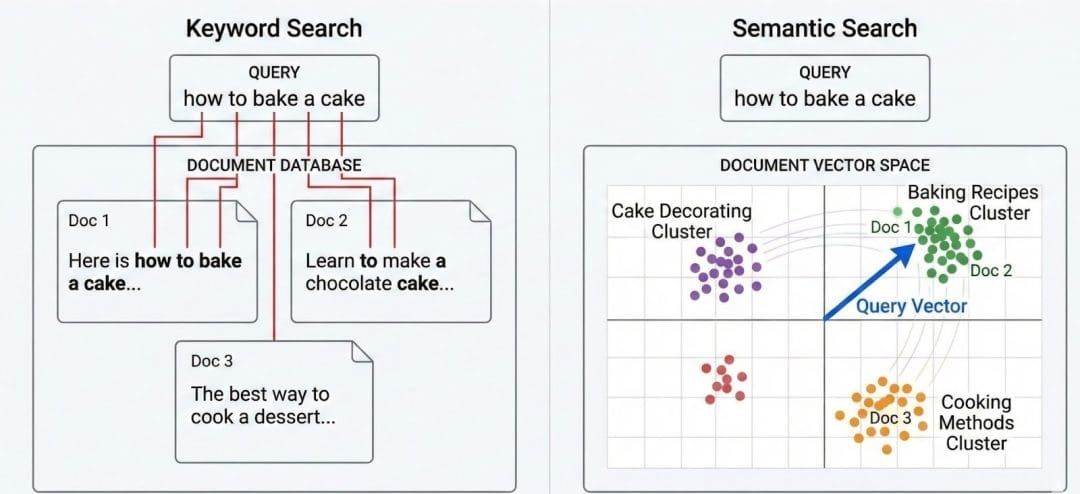
When “Totally different Phrases” Imply the Similar Factor

Let’s take a look at 2 easy queries:

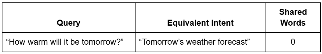
Q1: “How heat will or not it’s tomorrow?”

Q2: “Tomorrow’s climate forecast”

These sentences specific the identical intent — you’re asking in regards to the climate — however they share nearly no overlapping phrases.

A key phrase search engine ranks paperwork by shared phrases.

If there’s no shared token (“heat,” “forecast”), it might utterly miss the match.

That is known as an intent mismatch: lexical similarity (identical phrases) fails to seize semantic similarity (identical which means).

Even worse, paperwork stuffed with repeated question phrases can falsely seem extra related, even when they lack context.

---

Why TF-IDF and BM25 Fall Quick

TF-IDF (Time period Frequency–Inverse Doc Frequency) provides excessive scores to phrases that happen typically in a single doc however hardly ever throughout others.

It’s highly effective for distinguishing subjects, however brittle for which means.

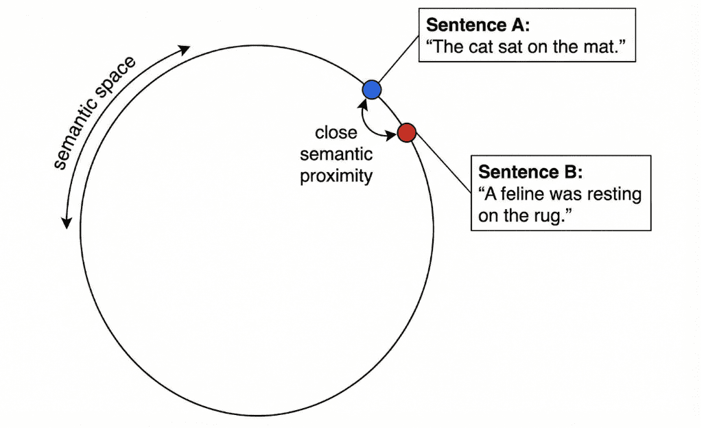
For instance, within the sentence:

“The cat sat on the mat,”
TF-IDF solely is aware of about floor tokens. It can not inform that “feline resting on carpet” means practically the identical factor.

BM25 (Finest Matching 25) improves rating through time period saturation and document-length normalization, however nonetheless essentially is determined by lexical overlap fairly than semantic which means.

---

The Price of Lexical Considering

Key phrase search struggles with:

• Synonyms: “AI” vs “Synthetic Intelligence”
• Paraphrases: “Repair the bug” vs “Resolve the difficulty”
• Polysemy: “Apple” (fruit) vs “Apple” (firm)
• Language flexibility: “Film” vs “Movie”

For people, these are trivially associated. For conventional algorithms, they’re fully completely different strings.

Instance:

Looking “how you can make my code run sooner” may not floor a doc titled “Python optimization suggestions” — regardless that it’s precisely what you want.

---

Why Which means Requires Geometry

Language is steady; which means exists on a spectrum, not in discrete phrase buckets.

So as a substitute of matching strings, what if we may plot their meanings in a high-dimensional area — the place related concepts sit shut collectively, even when they use completely different phrases?

That’s the leap from key phrase search to semantic search.

As a substitute of asking “Which paperwork share the identical phrases?” we ask:

“Which paperwork imply one thing related?”

And that’s exactly what embeddings and vector databases allow.

Now that you just perceive why keyword-based search fails, let’s discover how vector databases remedy this — by storing and evaluating which means, not simply phrases.

---

What Are Vector Databases and Why They Matter

Conventional databases are nice at dealing with structured information — numbers, strings, timestamps — issues that match neatly into tables and indexes.

However the true world isn’t that tidy. We take care of unstructured information: textual content, photographs, audio, movies, and paperwork that don’t have a predefined schema.

That’s the place vector databases are available in.

They retailer and retrieve semantic which means fairly than literal textual content.

As a substitute of looking out by key phrases, we search by ideas — via a steady, geometric illustration of information known as embeddings.

---

The Core Concept

Every bit of unstructured information — akin to a paragraph, picture, or audio clip — is handed via a mannequin (e.g., a SentenceTransformer or CLIP (Contrastive Language-Picture Pre-Coaching) mannequin), which converts it right into a vector (i.e., a listing of numbers).

These numbers seize semantic relationships: gadgets which can be conceptually related find yourself nearer collectively on this multi-dimensional area.

Instance: “vector database,” “semantic search,” and “retrieval-augmented technology” would possibly cluster close to one another, whereas “climate forecast” or “local weather information” type one other neighborhood.

Formally, every vector is a level in an N-dimensional area (the place N = mannequin’s embedding dimension, e.g., 384 or 768).

The distance between factors represents how associated they’re — cosine similarity, interior product, or Euclidean distance being the most typical measures.

---

Why This Issues

The great thing about vector databases is that they make which means searchable. As a substitute of doing a full textual content scan each time you ask a query, you exchange the query into its personal vector and discover neighboring vectors that signify related ideas.

This makes them the spine of:

• Semantic search: discover conceptually related outcomes
• Suggestions: discover “gadgets like this one”
• RAG pipelines: discover factual context for LLM solutions
• Clustering and discovery: group related content material collectively

---

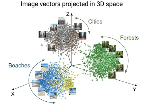
Instance 1: Organizing Pictures by Which means

Think about you’ve a set of trip photographs: seashores, mountains, forests, and cities.

As a substitute of sorting by file title or date taken, you utilize a imaginative and prescient mannequin to extract embeddings from every picture.

Every photograph turns into a vector encoding visible patterns akin to:

• dominant colours: blue ocean vs. inexperienced forest
• textures: sand vs. snow
• objects: buildings, bushes, waves

While you question “mountain surroundings”, the system converts your textual content right into a vector and compares it with all saved picture vectors.

These with the closest vectors (i.e., semantically related content material) are retrieved.

That is exactly how Google Photographs, Pinterest, and e-commerce visible search programs possible work internally.

---

Instance 2: Looking Throughout Textual content

Now contemplate a corpus of 1000’s of stories articles.

A conventional key phrase seek for “AI regulation in Europe” would possibly miss a doc titled “EU passes new AI security act” as a result of the precise phrases differ.

With vector embeddings, each queries and paperwork reside in the identical semantic area, so similarity is determined by which means — not actual phrases.

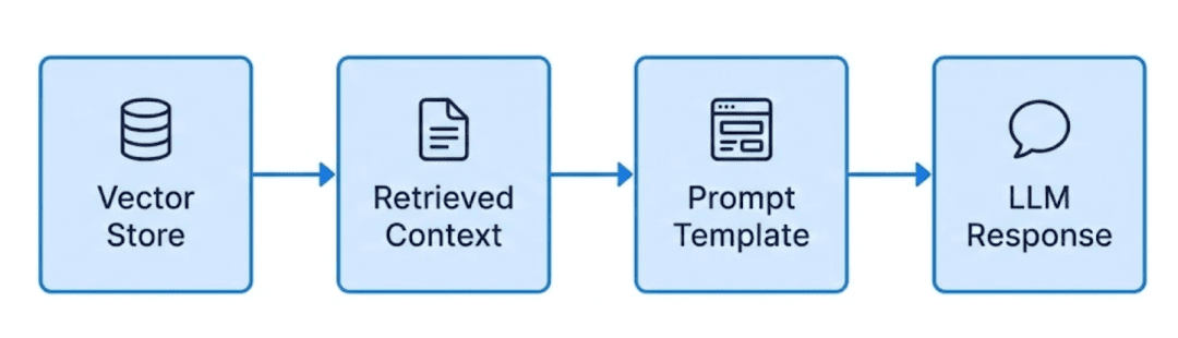
That is the inspiration of RAG (Retrieval-Augmented Technology) programs, the place retrieved passages (primarily based on embeddings) feed into an LLM to provide grounded solutions.

---

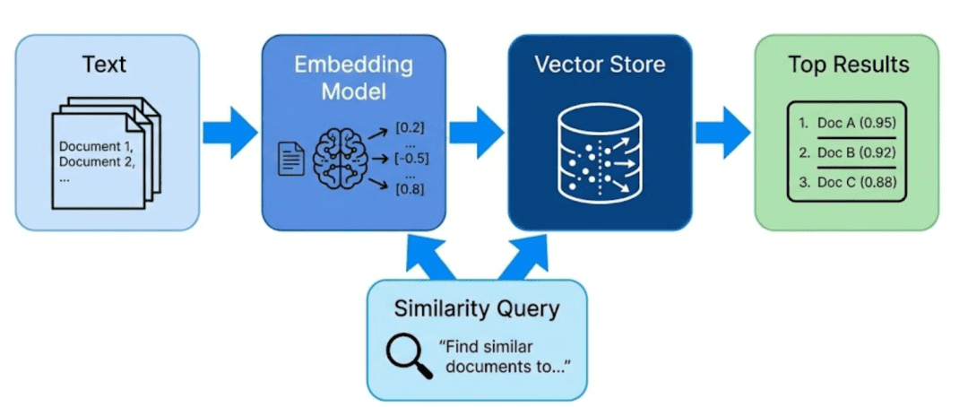
How It Works Conceptually

• Encoding: Convert uncooked content material (textual content, picture, and so on.) into dense numerical vectors
• Storing: Save these vectors and their metadata in a vector database
• Querying: Convert an incoming question right into a vector and discover nearest neighbors
• Returning: Retrieve each the matched embeddings and the unique information they signify

This final level is essential — a vector database doesn’t simply retailer vectors; it retains each embeddings and uncooked content material aligned.

In any other case, you’d discover “related” gadgets however haven’t any approach to present the consumer what these gadgets really have been.

Analogy:
Consider embeddings as coordinates, and the vector database as a map that additionally remembers the real-world landmarks behind every coordinate.

---

Why It’s a Large Deal

Vector databases bridge the hole between uncooked notion and reasoning.

They permit machines to:

• Perceive semantic closeness between concepts
• Generalize past actual phrases or literal matches
• Scale to thousands and thousands of vectors effectively utilizing Approximate Nearest Neighbor (ANN) search

You’ll implement that final half — ANN — in Lesson 2, however for now, it’s sufficient to know that vector databases make which means each storable and searchable.

Transition:

Now that what vector databases are and why they’re so highly effective, let’s take a look at how we mathematically signify which means itself — with embeddings.

---

Understanding Embeddings: Turning Language into Geometry

If a vector database is the mind’s reminiscence, embeddings are the neurons that maintain which means.

At a excessive stage, an embedding is only a record of floating-point numbers — however every quantity encodes a latent function discovered by a mannequin.

Collectively, these options signify the semantics of an enter: what it talks about, what ideas seem, and the way these ideas relate.

So when two texts imply the identical factor — even when they use completely different phrases — their embeddings lie shut collectively on this high-dimensional area.

🧠 Consider embeddings as “which means coordinates.”
The nearer two factors are, the extra semantically alike their underlying texts are.

---

Why Do We Want Embeddings?

Conventional key phrase search works by counting shared phrases.

However language is versatile — the identical thought may be expressed in lots of varieties:

Embeddings repair this by mapping each sentences to close by vectors — the geometric sign of shared which means.

---

How Embeddings Work (Conceptually)

Once we feed textual content into an embedding mannequin, it outputs a vector like:

[0.12, -0.45, 0.38, ..., 0.09]

Every dimension encodes latent attributes akin to matter, tone, or contextual relationships.

For instance:

• “banana” and “apple” would possibly share excessive weights on a fruit dimension
• “AI mannequin” and “neural community” would possibly align on a expertise dimension

When visualized (e.g., with PCA or t-SNE), semantically related gadgets cluster collectively — you’ll be able to actually see which means from patterns.

---

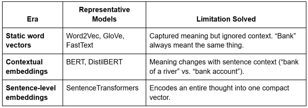
From Static to Contextual to Sentence-Stage Embeddings

Embeddings didn’t all the time perceive context.

They advanced via 3 main eras — every addressing a key limitation.

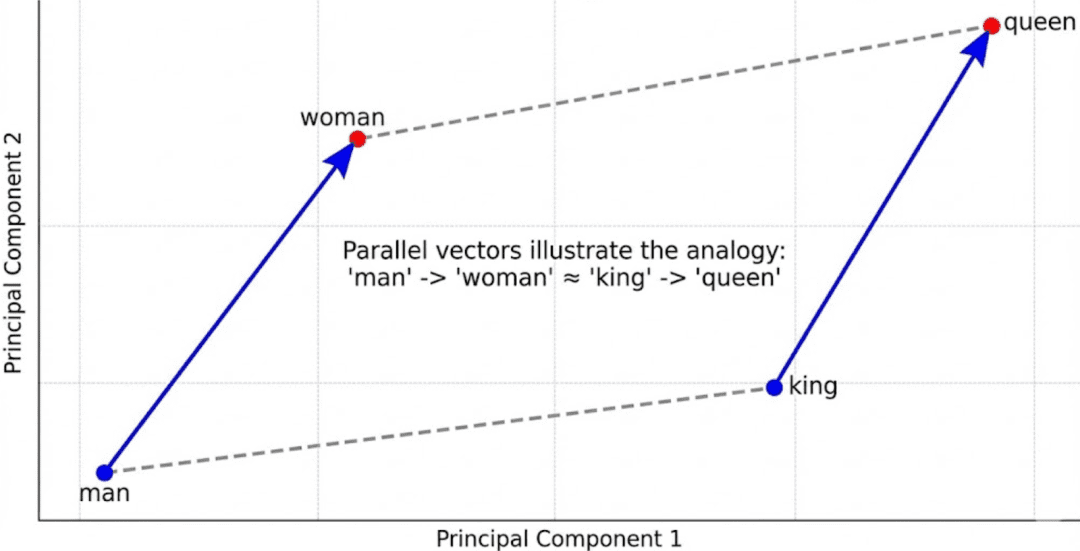
Instance: Word2Vec Analogies

Early fashions akin to Word2Vec captured fascinating linear relationships:

King - Man + Lady ≈ Queen
Paris - France + Italy ≈ Rome

These confirmed that embeddings may signify conceptual arithmetic.

However Word2Vec assigned just one vector per phrase — so it failed for polysemous phrases akin to desk (“spreadsheet” vs. “furnishings”).

Callout:
Static embeddings = one vector per phrase → no context.
Contextual embeddings = completely different vectors per sentence → true understanding.

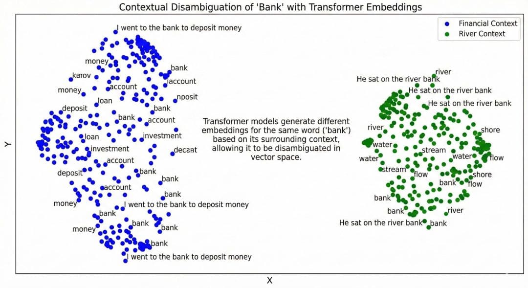
BERT and the Transformer Revolution

Transformers launched contextualized embeddings through self-attention.

As a substitute of treating phrases independently, the mannequin appears to be like at surrounding phrases to deduce which means.

BERT (Bidirectional Encoder Representations from Transformers) makes use of 2 coaching targets:

• Masked Language Modeling (MLM): randomly hides phrases and predicts them utilizing context.
• Subsequent Sentence Prediction (NSP): determines whether or not two sentences observe one another.

This bidirectional understanding made embeddings context-aware — the phrase “financial institution” now has distinct vectors relying on utilization.

Sentence Transformers

Sentence Transformers (constructed on BERT and DistilBERT) lengthen this additional — they generate one embedding per sentence or paragraph fairly than per phrase.

That’s precisely what your mission makes use of:
all-MiniLM-L6-v2, a light-weight, high-quality mannequin that outputs 384-dimensional sentence embeddings.

Every embedding captures the holistic intent of a sentence — excellent for semantic search and RAG.

---

How This Maps to Your Code

In pyimagesearch/config.py, you outline:

EMBED_MODEL_NAME = "sentence-transformers/all-MiniLM-L6-v2"

That line tells your pipeline which mannequin to load when producing embeddings.

The whole lot else (batch measurement, normalization, and so on.) is dealt with by helper features in pyimagesearch/embeddings_utils.py.

Let’s unpack how that occurs.

Loading the Mannequin

from sentence_transformers import SentenceTransformer

def get_model(model_name=config.EMBED_MODEL_NAME):
    return SentenceTransformer(model_name)

This fetches a pretrained SentenceTransformer from Hugging Face, hundreds it as soon as, and returns a ready-to-use encoder.

Producing Embeddings

def generate_embeddings(texts, mannequin=None, batch_size=16, normalize=True):
    embeddings = mannequin.encode(
        texts, batch_size=batch_size, show_progress_bar=True,
        convert_to_numpy=True, normalize_embeddings=normalize
    )
    return embeddings

Every textual content line out of your corpus (information/enter/corpus.txt) is remodeled right into a 384-dimensional vector.

Normalization ensures all vectors lie on a unit sphere — that’s why later, cosine similarity turns into only a dot product.

Tip: Cosine similarity measures angle, not size.
L2 normalization retains all embeddings equal-length, so solely path (which means) issues.

---

Why Embeddings Cluster Semantically

When plotted (utilizing PCA (principal element evaluation) or t-SNE (t-distributed stochastic neighbor embedding)), embeddings from related subjects type clusters:

• “vector database,” “semantic search,” “HNSW” (hierarchical navigable small world) → one cluster
• “normalization,” “cosine similarity” → one other

That occurs as a result of embeddings are skilled with contrastive targets — pushing semantically shut examples collectively and unrelated ones aside.

You’ve now seen what embeddings are, how they advanced, and the way your code turns language into geometry — factors in a high-dimensional area the place which means lives.

Subsequent, let’s deliver all of it collectively.

We’ll stroll via the complete implementation — from configuration and utilities to the principle driver script — to see precisely how this semantic search pipeline works end-to-end.

---

Would you want instant entry to three,457 photographs curated and labeled with hand gestures to coach, discover, and experiment with … at no cost? Head over to Roboflow and get a free account to seize these hand gesture photographs.

---

Configuring Your Growth Atmosphere

To observe this information, you have to set up a number of Python libraries for working with semantic embeddings and textual content processing.

The core dependencies are:

$ pip set up sentence-transformers==2.7.0
$ pip set up numpy==1.26.4  
$ pip set up wealthy==13.8.1

---

Verifying Your Set up

You possibly can confirm the core libraries are correctly put in by operating:

from sentence_transformers import SentenceTransformer
import numpy as np
from wealthy import print

mannequin = SentenceTransformer('all-MiniLM-L6-v2')
print("Atmosphere setup full!")

Word: The sentence-transformers library will routinely obtain the embedding mannequin on first use, which can take a couple of minutes relying in your web connection.

---

Want Assist Configuring Your Growth Atmosphere?

All that mentioned, are you:

• Quick on time?
• Studying in your employer’s administratively locked system?
• Eager to skip the effort of combating with the command line, bundle managers, and digital environments?
• Able to run the code instantly in your Home windows, macOS, or Linux system?

Then be a part of PyImageSearch College in the present day!

Acquire entry to Jupyter Notebooks for this tutorial and different PyImageSearch guides pre-configured to run on Google Colab’s ecosystem proper in your internet browser! No set up required.

And better of all, these Jupyter Notebooks will run on Home windows, macOS, and Linux!

---

Implementation Walkthrough: Configuration and Listing Setup

Your config.py file acts because the spine of this complete RAG sequence.

It defines the place information lives, how fashions are loaded, and the way completely different pipeline elements (embeddings, indexes, prompts) speak to one another.

Consider it as your mission’s single supply of fact — modify paths or fashions right here, and each script downstream stays constant.

---

Setting Up Core Directories

from pathlib import Path
import os

BASE_DIR = Path(__file__).resolve().dad or mum.dad or mum
DATA_DIR = BASE_DIR / "information"
INPUT_DIR = DATA_DIR / "enter"
OUTPUT_DIR = DATA_DIR / "output"
INDEX_DIR = DATA_DIR / "indexes"
FIGURES_DIR = DATA_DIR / "figures"

Every fixed defines a key working folder.

• BASE_DIR: dynamically finds the mission’s root, irrespective of the place you run the script from
• DATA_DIR: teams all mission information below one roof
• INPUT_DIR: your supply textual content (corpus.txt) and non-compulsory metadata
• OUTPUT_DIR: cached artifacts akin to embeddings and PCA (principal element evaluation) projections
• INDEX_DIR: FAISS (Fb AI Similarity Search) indexes you’ll construct in Half 2
• FIGURES_DIR: visualizations akin to 2D semantic plots

TIP: Centralizing all paths prevents complications later when switching between native, Colab, or AWS environments.

---

Corpus Configuration

_CORPUS_OVERRIDE = os.getenv("CORPUS_PATH")
_CORPUS_META_OVERRIDE = os.getenv("CORPUS_META_PATH")
CORPUS_PATH = Path(_CORPUS_OVERRIDE) if _CORPUS_OVERRIDE else INPUT_DIR / "corpus.txt"
CORPUS_META_PATH = Path(_CORPUS_META_OVERRIDE) if _CORPUS_META_OVERRIDE else INPUT_DIR / "corpus_metadata.json"

This allows you to override corpus recordsdata through atmosphere variables — helpful whenever you wish to check completely different datasets with out modifying the code.

As an illustration:

export CORPUS_PATH=/mnt/information/new_corpus.txt

Now, all scripts routinely choose up that new file.

---

Embedding and Mannequin Artifacts

EMBEDDINGS_PATH = OUTPUT_DIR / "embeddings.npy"
METADATA_ALIGNED_PATH = OUTPUT_DIR / "metadata_aligned.json"
DIM_REDUCED_PATH = OUTPUT_DIR / "pca_2d.npy"
FLAT_INDEX_PATH = INDEX_DIR / "faiss_flat.index"
HNSW_INDEX_PATH = INDEX_DIR / "faiss_hnsw.index"
EMBED_MODEL_NAME = "sentence-transformers/all-MiniLM-L6-v2"

Right here, we outline the semantic artifacts this pipeline will create and reuse.

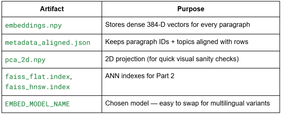
Why all-MiniLM-L6-v2?

It’s light-weight (384 dimensions), quick, and top quality for brief passages — excellent for demos.

Later, you’ll be able to simply exchange it with a multilingual or domain-specific mannequin by altering this single variable.

---

Normal Settings

SEED = 42
DEFAULT_TOP_K = 5
SIM_THRESHOLD = 0.35

These constants management experiment repeatability and rating logic.

• SEED: retains PCA and ANN reproducible
• DEFAULT_TOP_K: units what number of neighbors to retrieve for queries
• SIM_THRESHOLD: acts as a free cutoff to disregard extraordinarily weak matches

---

Non-obligatory: Immediate Templates for RAG

Although not but utilized in Lesson 1, the config already prepares the RAG basis:

STRICT_SYSTEM_PROMPT = (
    "You're a concise assistant. Use ONLY the supplied context."
    " If the reply will not be contained verbatim or explicitly, say you have no idea."
)
SYNTHESIZING_SYSTEM_PROMPT = (
    "You're a concise assistant. Rely ONLY on the supplied context, however you MAY synthesize"
    " a solution by combining or paraphrasing the details current."
)
USER_QUESTION_TEMPLATE = "Person Query: {query}nAnswer:"
CONTEXT_HEADER = "Context:"

This anticipates how the retriever (vector database) will later feed context chunks right into a language mannequin.

In Half 3, you’ll use these templates to assemble dynamic prompts in your RAG pipeline.

---

Last Contact

for d in (OUTPUT_DIR, INDEX_DIR, FIGURES_DIR):
    d.mkdir(mother and father=True, exist_ok=True)

A small however highly effective line — ensures all directories exist earlier than writing any recordsdata.

You’ll by no means once more get the “No such file or listing” error throughout your first run.

In abstract, config.py defines the mission’s constants, artifacts, and mannequin parameters — conserving all the pieces centralized, reproducible, and RAG-ready.

Subsequent, we’ll transfer to embeddings_utils.py, the place you’ll load the corpus, generate embeddings, normalize them, and persist the artifacts.

---

Embedding Utilities (embeddings_utils.py)

---

Overview

This module powers all the pieces you’ll do in Lesson 1. It gives reusable, modular features for:

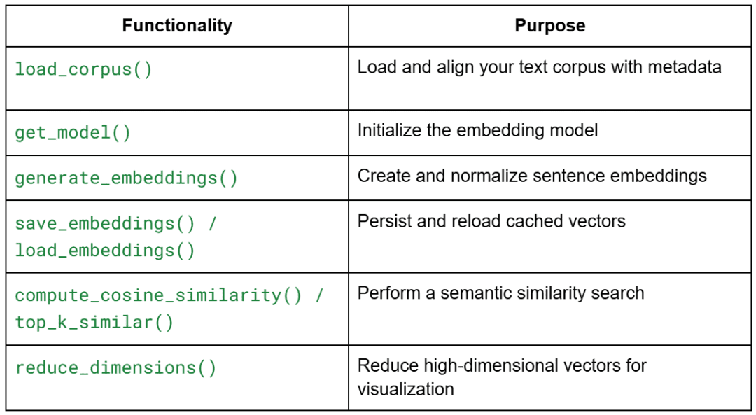
Every operate is intentionally stateless — you’ll be able to plug them into different initiatives later with out modification.

---

Loading the Corpus

def load_corpus(corpus_path=CORPUS_PATH, meta_path=CORPUS_META_PATH):
    with open(corpus_path, "r", encoding="utf-8") as f:
        texts = [line.strip() for line in f if line.strip()]
    if meta_path.exists():
        import json; metadata = json.load(open(meta_path, "r", encoding="utf-8"))
    else:
        metadata = []
    if len(metadata) != len(texts):
        metadata = [{"id": f"p{idx:02d}", "topic": "unknown", "tokens_est": len(t.split())} for idx, t in enumerate(texts)]
    return texts, metadata

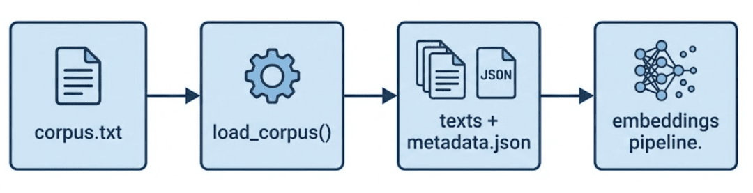
That is the start line of your information circulation.

It reads every non-empty paragraph out of your corpus (information/enter/corpus.txt) and pairs it with metadata entries.

Why It Issues

• Ensures alignment — every embedding all the time maps to its unique textual content
• Routinely repairs metadata if mismatched or lacking
• Prevents silent information drift throughout re-runs

TIP: In later classes, this alignment ensures the top-k search outcomes may be traced again to their paragraph IDs or subjects.

---

Loading the Embedding Mannequin

from sentence_transformers import SentenceTransformer

def get_model(model_name=EMBED_MODEL_NAME):
    return SentenceTransformer(model_name)

This operate centralizes mannequin loading.

As a substitute of hard-coding the mannequin all over the place, you name get_model() as soon as — making the remainder of your pipeline model-agnostic.

Why This Sample

• Let’s you swap fashions simply (e.g., multilingual or domain-specific)
• Retains the motive force script clear
• Prevents re-initializing the mannequin repeatedly (you’ll reuse the identical occasion)

Mannequin perception:
all-MiniLM-L6-v2 has 22 M parameters and produces 384-dimensional embeddings.

It’s quick sufficient for native demos but semantically wealthy sufficient for clustering and similarity rating.

---

Producing Embeddings

import numpy as np

def generate_embeddings(texts, mannequin=None, batch_size: int = 16, normalize: bool = True):
    if mannequin is None: mannequin = get_model()
    embeddings = mannequin.encode(
        texts,
        batch_size=batch_size,
        show_progress_bar=True,
        convert_to_numpy=True,
        normalize_embeddings=normalize
    )
    if normalize:
        norms = np.linalg.norm(embeddings, axis=1, keepdims=True)
        norms[norms == 0] = 1.0
        embeddings = embeddings / norms
    return embeddings

That is the center of Lesson 1 — changing human language into geometry.

What Occurs Step by Step

1. Encode textual content: Every sentence turns into a dense vector of 384 floats
2. Normalize: Divides every vector by its L2 norm so it lies on a unit hypersphere
3. Return NumPy array: Form → (n_paragraphs × 384)

Why Normalization?

As a result of cosine similarity is determined by vector path, not size.

L2 normalization makes cosine = dot product — sooner and easier for rating.

Psychological mannequin:
Every paragraph now “lives” someplace on the floor of a sphere the place close by factors share related which means.

---

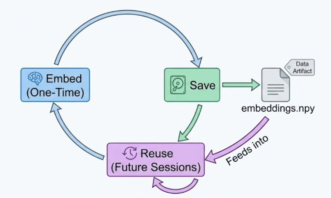
Saving and Loading Embeddings

import json

def save_embeddings(embeddings, metadata, emb_path=EMBEDDINGS_PATH, meta_out_path=METADATA_ALIGNED_PATH):
    np.save(emb_path, embeddings)
    json.dump(metadata, open(meta_out_path, "w", encoding="utf-8"), indent=2)

def load_embeddings(emb_path=EMBEDDINGS_PATH, meta_out_path=METADATA_ALIGNED_PATH):
    emb = np.load(emb_path)
    meta = json.load(open(meta_out_path, "r", encoding="utf-8"))
    return emb, meta

Caching is important after you have costly embeddings. These two helpers retailer and reload them in seconds.

Why Each .npy and .json?

• .npy: quick binary format for numeric information
• .json: human-readable mapping of metadata to embeddings

Good follow:
By no means modify metadata_aligned.json manually — it ensures row consistency between textual content and embeddings.

---

Computing Similarity and Rating

def compute_cosine_similarity(vec, matrix):
    return matrix @ vec

def top_k_similar(query_emb, emb_matrix, okay=DEFAULT_TOP_K):
    sims = compute_cosine_similarity(query_emb, emb_matrix)
    idx = np.argpartition(-sims, okay)[:k]
    idx = idx[np.argsort(-sims[idx])]
    return idx, sims[idx]

These two features remodel your embeddings right into a semantic search engine.

How It Works

• compute_cosine_similarity: performs a quick dot-product of a question vector towards the embedding matrix
• top_k_similar: picks the top-okay outcomes with out sorting all N entries — environment friendly even for giant corpora

Analogy:
Consider it like Google search, however as a substitute of matching phrases, it measures which means overlap through vector angles.

Complexity:
O(N × D) per question — acceptable for small datasets, however this units up the motivation for ANN indexing in Lesson 2.

---

Decreasing Dimensions for Visualization

from sklearn.decomposition import PCA

def reduce_dimensions(embeddings, n_components=2, seed=42):
    pca = PCA(n_components=n_components, random_state=seed)
    return pca.fit_transform(embeddings)

Why PCA?

• People can’t visualize 384-D area
• PCA compresses to 2-D whereas preserving the biggest variance instructions
• Excellent for sanity-checking that semantic clusters look affordable

Bear in mind: You’ll nonetheless carry out searches in 384-D — PCA is for visualization solely.

At this level, you’ve:

• Clear corpus + metadata alignment
• A working embedding generator
• Normalized vectors prepared for cosine similarity
• Non-obligatory visualization through PCA

All that is still is to attach these utilities in your foremost driver script (01_intro_to_embeddings.py), the place we’ll orchestrate embedding creation, semantic search, and visualization.

---

Driver Script Walkthrough (01_intro_to_embeddings.py)

The motive force script doesn’t introduce new algorithms — it wires collectively all of the modular utilities you simply constructed.

Let’s undergo it piece by piece so that you perceive not solely what occurs however why every half belongs the place it does.

---

Imports and Setup

import numpy as np
from wealthy import print
from wealthy.desk import Desk

from pyimagesearch import config
from pyimagesearch.embeddings_utils import (
    load_corpus,
    generate_embeddings,
    save_embeddings,
    load_embeddings,
    get_model,
    top_k_similar,
    reduce_dimensions,
)

Rationalization

• You’re importing helper features from embeddings_utils.py and configuration constants from config.py.
• wealthy is used for pretty-printing output tables within the terminal — provides colour and formatting for readability.
• The whole lot else (numpy, reduce_dimensions, and so on.) was already lined; we’re simply combining them right here.

---

Guaranteeing Embeddings Exist or Rebuilding Them

def ensure_embeddings(pressure: bool = False):
    if config.EMBEDDINGS_PATH.exists() and never pressure:
        emb, meta = load_embeddings()
        texts, _ = load_corpus()
        return emb, meta, texts
    texts, meta = load_corpus()
    mannequin = get_model()
    emb = generate_embeddings(texts, mannequin=mannequin, batch_size=16, normalize=True)
    save_embeddings(emb, meta)
    return emb, meta, texts

What This Perform Does

That is your entry checkpoint — it ensures you all the time have embeddings earlier than doing anything.

• If cached .npy and .json recordsdata exist → merely load them (no recomputation)
• In any other case → learn the corpus, generate embeddings, save them, and return

Why It Issues

• Saves you from recomputing embeddings each run (an enormous time saver)
• Retains constant mapping between textual content ↔ embedding throughout periods
• The pressure flag helps you to rebuild from scratch for those who change fashions or information

TIP: In manufacturing, you’d make this a CLI (command line interface) flag like --rebuild in order that automation scripts can set off a full re-embedding if wanted.

---

Exhibiting Nearest Neighbors (Semantic Search Demo)

def show_neighbors(embeddings: np.ndarray, texts, mannequin, queries):
    print("[bold cyan]nSemantic Similarity Examples[/bold cyan]")
    for q in queries:
        q_emb = mannequin.encode([q], convert_to_numpy=True, normalize_embeddings=True)[0]
        idx, scores = top_k_similar(q_emb, embeddings, okay=5)
        desk = Desk(title=f"Question: {q}")
        desk.add_column("Rank")
        desk.add_column("Rating", justify="proper")
        desk.add_column("Textual content (truncated)")
        for rank, (i, s) in enumerate(zip(idx, scores), begin=1):
            snippet = texts[i][:100] + ("..." if len(texts[i]) > 100 else "")
            desk.add_row(str(rank), f"{s:.3f}", snippet)
        print(desk)

Step-by-Step

• Loop over every natural-language question (e.g., “Clarify vector databases”)
• Encode it right into a vector through the identical mannequin — guaranteeing semantic consistency
• Retrieve top-okay related paragraphs through cosine similarity.
• Render the end result as a formatted desk with rank, rating, and a brief snippet

What This Demonstrates

• It’s your first actual semantic search — no indexing but, however full meaning-based retrieval
• Exhibits how “nearest neighbors” are decided by semantic closeness, not phrase overlap
• Units the stage for ANN acceleration in Lesson 2

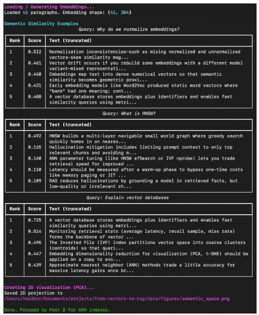
OBSERVATION: Even with solely 41 paragraphs, the search feels “clever” as a result of the embeddings seize concept-level similarity.

---

Visualizing the Embedding House

def visualize(embeddings: np.ndarray):
    coords = reduce_dimensions(embeddings, n_components=2)
    np.save(config.DIM_REDUCED_PATH, coords)
    strive:
        import matplotlib.pyplot as plt
        fig_path = config.FIGURES_DIR / "semantic_space.png"
        plt.determine(figsize=(6, 5))
        plt.scatter(coords[:, 0], coords[:, 1], s=20, alpha=0.75)
        plt.title("PCA Projection of Corpus Embeddings")
        plt.tight_layout()
        plt.savefig(fig_path, dpi=150)
        print(f"Saved 2D projection to {fig_path}")
    besides Exception as e:
        print(f"[yellow]Couldn't generate plot: {e}[/yellow]")

Why Visualize?

Visualization makes summary geometry tangible.

PCA compresses 384 dimensions into 2, so you’ll be able to see whether or not associated paragraphs are clustering collectively.

Implementation Notes

• Shops projected coordinates (pca_2d.npy) for re-use in Lesson 2.
• Gracefully handles environments with out show backends (e.g., distant SSH (Safe Shell)).
• Transparency (alpha=0.75) helps overlapping clusters stay readable.

---

Principal Orchestration Logic

def foremost():
    print("[bold magenta]Loading / Producing Embeddings...[/bold magenta]")
    embeddings, metadata, texts = ensure_embeddings()
    print(f"Loaded {len(texts)} paragraphs. Embedding form: {embeddings.form}")

    mannequin = get_model()

    sample_queries = [
        "Why do we normalize embeddings?",
        "What is HNSW?",
        "Explain vector databases",
    ]
    show_neighbors(embeddings, texts, mannequin, sample_queries)

    print("[bold magenta]nCreating 2D visualization (PCA)...[/bold magenta]")
    visualize(embeddings)

    print("[green]nDone. Proceed to Publish 2 for ANN indexes.n[/green]")


if __name__ == "__main__":
    foremost()

Move Defined

• Begin → load or construct embeddings
• Run semantic queries and present high outcomes
• Visualize 2D projection
• Save all the pieces for the subsequent lesson

The print colours (magenta, cyan, inexperienced) assist readers observe the stage development clearly when operating within the terminal.

---

Instance Output (Anticipated Terminal Run)

While you run:

python 01_intro_to_embeddings.py

It’s best to see one thing like this in your terminal:

---

What You’ve Constructed So Far

• A mini semantic search engine that retrieves paragraphs by which means, not key phrase
• Persistent artifacts (embeddings.npy, metadata_aligned.json, pca_2d.npy)
• Visualization of idea clusters that proves embeddings seize semantics

This closes the loop for Lesson 1: Understanding Vector Databases and Embeddings — you’ve applied all the pieces as much as the baseline semantic search.

---

---

Abstract

On this lesson, you constructed the inspiration for understanding how machines signify which means.

You started by revisiting the restrictions of keyword-based search — the place two sentences can specific the identical intent but stay invisible to at least one one other as a result of they share few widespread phrases. From there, you explored how embeddings remedy this downside by mapping language right into a steady vector area the place proximity displays semantic similarity fairly than mere token overlap.

You then discovered how trendy embedding fashions (e.g., SentenceTransformers) generate these dense numerical vectors. Utilizing the all-MiniLM-L6-v2 mannequin, you remodeled each paragraph in your handcrafted corpus right into a 384-dimensional vector — a compact illustration of its which means. Normalization ensured that each vector lay on the unit sphere, making cosine similarity equal to a dot product.

With these embeddings in hand, you carried out your first semantic similarity search. As a substitute of counting shared phrases, you in contrast the path of which means between sentences and noticed how conceptually associated passages naturally rose to the highest of your rankings. This hands-on demonstration illustrated the facility of geometric search — the bridge from uncooked language to understanding.

Lastly, you visualized this semantic panorama utilizing PCA, compressing lots of of dimensions down to 2. The ensuing scatter plot revealed emergent clusters: paragraphs about normalization, approximate nearest neighbors, and vector databases fashioned their very own neighborhoods. It’s a visible affirmation that the mannequin has captured real construction in which means.

By the tip of this lesson, you didn’t simply study what embeddings are — you noticed them in motion. You constructed a small however full semantic engine: loading information, encoding textual content, looking out by which means, and visualizing relationships. These artifacts now function the enter for the subsequent stage of the journey, the place you’ll make search actually scalable by constructing environment friendly Approximate Nearest Neighbor (ANN) indexes with FAISS.

In Lesson 2, you’ll learn to velocity up similarity search from 1000’s of comparisons to milliseconds — the important thing step that turns your semantic area right into a production-ready vector database.

---

Quotation Data

Singh, V. “TF-IDF vs. Embeddings: From Key phrases to Semantic Search,” PyImageSearch, P. Chugh, S. Huot, A. Sharma, and P. Thakur, eds., 2026, https://pyimg.co/msp43

@incollection{Singh_2026_tf-idf-vs-embeddings-from-keywords-to-semantic-search,
  writer = {Vikram Singh},
  title = {{TF-IDF vs. Embeddings: From Key phrases to Semantic Search}},
  booktitle = {PyImageSearch},
  editor = {Puneet Chugh and Susan Huot and Aditya Sharma and Piyush Thakur},
  yr = {2026},
  url = {https://pyimg.co/msp43},
}

---

To obtain the supply code to this put up (and be notified when future tutorials are revealed right here on PyImageSearch), merely enter your electronic mail handle within the type beneath!

The put up TF-IDF vs. Embeddings: From Key phrases to Semantic Search appeared first on PyImageSearch.