

November 20, 2020
Neural tangent kernels are a great tool for understanding neural community coaching and implicit regularization in gradient descent. However it’s not the simplest idea to wrap your head round. The paper that I discovered to have been most helpful for me to develop an understanding is that this one:
On this submit I’ll illustrate the idea of neural tangent kernels by means of a easy 1D regression instance. Please be at liberty to peruse the google colab pocket book I used to make these plots.
Instance 1: Warming up
Let’s begin from a really boring case start with. For example we’ve got a operate outlined over integers between -10 and 20. We parametrize our operate as a look-up desk, that’s the worth of the operate $f(i)$ at every integer $i$ is described by a separate parameter $theta_i = f(i)$. I am initializing the parameters of this operate as $theta_i = 3i+2$. The operate is proven by the black dots beneath:
Now, let’s take into account what occurs if we observe a brand new datapoint, $(x, y) =(10, 50)$, proven by the blue cross. We’ll take a gradient descent step updating $theta$. For example we use the squared error loss operate $(f(10; theta) – 50)^2$ and a studying charge $eta=0.1$. As a result of the operate’s worth at $x=10$ solely is dependent upon one of many parameter $theta_10$, solely this parameter can be up to date. The remainder of the parameters, and subsequently the remainder of the operate values stay unchanged. The pink arrows illustrate the way in which operate values transfer in a single gradient descent step: Most values do not transfer in any respect, solely one among them strikes nearer to the noticed information. Therefore just one seen pink arrow.
Nonetheless, in machine studying we not often parametrize capabilities as lookup tables of particular person operate values. This parametrization is fairly ineffective because it would not permit you to interpolate not to mention extrapolate to unseen information. Let’s examine what occurs in a extra acquainted mannequin: linear regression.
Instance 2: Linear operate
Let’s now take into account the linear operate $f(x, theta) = theta_1 x + theta_2$. I initialize the parameters to $theta_1=3$ and $theta_2=1$, so at initialisation, I’ve precisely the identical operate over integers as I had within the first instance. Let us take a look at what occurs to this operate as I replace $theta$ by performing single gradient descent step incorporating the commentary $(x, y) =(10, 50)$ as earlier than. Once more, pink arrows are present how operate values transfer:
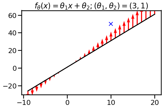
Whoa! What is going on on now? Since particular person operate values are now not independently parametrized, we won’t transfer them independently. The mannequin binds them collectively by means of its international parameters $theta_1$ and $theta_2$. If we need to transfer the operate nearer to the specified output $y=50$ at location $x=10$ the operate values elsewhere have to vary, too.
On this case, updating the operate with an commentary at $x=10$ modifications the operate worth distant from the commentary. It even modifications the operate worth in the wrong way than what one would count on.. This might sound a bit bizarre, however that is actually how linear fashions work.
Now we’ve got a bit of little bit of background to start out speaking about this neural tangent kernel factor.
Meet the neural tangent kernel
Given a operate $f_theta(x)$ which is parametrized by $theta$, its neural tangent kernel $k_theta(x, x’)$ quantifies how a lot the operate’s worth at $x$ modifications as we take an infinitesimally small gradient step in $theta$ incorporating a brand new commentary at $x’$. One other approach of phrasing that is: $ok(x, x’)$ measures how delicate the operate worth at $x$ is to prediction errors at $x’$.
Within the plots earlier than, the scale of the pink arrows at every location $x$ got by the next equation:
$$
eta tilde{ok}_theta(x, x’) = fleft(x, theta + eta frac{f_theta(x’)}{dtheta}proper) – f(x, theta)
$$
In neural community parlance, that is what is going on on: The loss operate tells me to extend the operate worth $f_theta(x’)$. I back-propagate this by means of the community to see what change in $theta$ do I’ve to make to realize this. Nonetheless, transferring $f_theta(x’)$ this manner additionally concurrently strikes $f_theta(x)$ at different areas $x neq x’$. $tilde{ok}_theta(x, x’)$ expresses by how a lot.
The neural kernel is mainly one thing just like the restrict of $tilde{ok}$ in because the stepsize turns into infinitesimally small. Specifically:
$$
ok(x, x’) = lim_{eta rightarrow 0} frac{fleft(x, theta + eta frac{df_theta(x’)}{dtheta}proper) – f(x, theta)}{eta}
$$
Utilizing a 1st order Taylor growth of $f_theta(x)$, it’s potential to point out that
$$
k_theta(x, x’) = leftlangle frac{df_theta(x)}{dtheta} , frac{f_theta(x’)}{dtheta} rightrangle
$$
As homework for you: discover $ok(x, x’)$ and/or $tilde{ok}(x, x’)$ for a set $eta$ within the linear mannequin within the pervious instance. Is it linear? Is it one thing else?
Observe that it is a completely different derivation from what’s within the paper (which begins from steady differential equation model of gradient descent).
Now, I am going to return to the examples for instance two extra essential property of this kernel: sensitivity to parametrization, and modifications throughout coaching.
Instance 3: Reparametrized linear mannequin
It is well-known that neural networks may be repararmetized in ways in which do not change the precise output of the operate, however which can result in variations in how optimization works. Batchnorm is a well known instance of this. Can we see the impact of reparametrization within the neural tangent kernel? Sure we are able to. Let us take a look at what occurs if I reparametrize the linear operate I used within the second instance as:
$$
f_theta(x) = theta_1 x + colour{blue}{10cdot}theta_2
$$
however now with parameters $theta_1=3, theta_2=colour{blue}{0.1}$. I highlighted in blue what modified. The operate itself, at initialization is identical since $10 * 0.1 = 1$. The operate class is identical, too, as I can nonetheless implement arbitrary linear capabilities. Nonetheless, after we have a look at the impact of a single gradient step, we see that the operate modifications in a different way when gradient descent is carried out on this parametrisation.
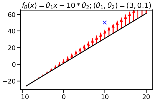
On this parametization, it turned simpler for gradient descent to push the entire operate up by a continuing, whereas within the earlier parametrisation it determined to vary the slope. What this demonstrates is that the neural tangent kernel $k_theta(x, x’)$ is delicate to reparametrization.
Instance 4: tiny radial foundation operate community
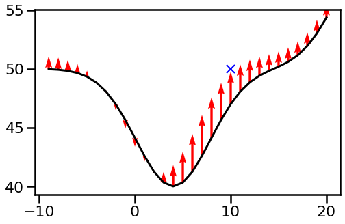
Whereas the linear fashions could also be good illustration, let us take a look at what $k_theta(x, x’)$ appears to be like like in a nonlinear mannequin. Right here, I am going to take into account a mannequin with two squared exponential foundation capabilities:
$$
f_theta(x) = theta_1 expleft(-frac{(x – theta_2)^2}{30}proper) + theta_3 expleft(-frac{(x – theta_4)^2}{30}proper) + theta_5,
$$
with preliminary parameter values $(theta_1, theta_2, theta_3, theta_4, theta_5) = (4.0, -10.0, 25.0, 10.0, 50.0)$. These are chosen considerably arbitrarily and to make the end result visually interesting:
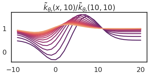
We are able to visualise the operate $tilde{ok}_theta(x, 10)$ instantly, relatively than plotting it on prime the operate. Right here I additionally normalize it by dividing by $tilde{ok}_theta(10, 10)$.
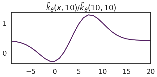
What we are able to see is that this begins to look a bit like a kernel operate in that it has larger values close to $10$ and reduces as you go farther away. Nonetheless, a number of issues are price noting: the utmost of this kernel operate will not be at $x=1o$, however at $x=7$. It means, that the operate worth $f(7)$ modifications extra in response to an commentary at $x’=10$ than the worth $f(10)$. Secondly, there are some damaging values. On this case the earlier determine supplies a visible reason why: we are able to enhance the operate worth at $x=10$ by pushing the valley centred at $theta_1=4$ away from it, to the left. This parameter change in flip decreases operate values on the left-hand wall of the valley. Third, the kernel operate converges to a constructive fixed at its tails – that is due to the offset $theta_5$.
Instance 5: Adjustments as we prepare
Now I will illustrate one other essential property of the neural tangent kernel: normally, the kernel is dependent upon the parameter worth $theta$, and subsequently it modifications because the mannequin is skilled. Right here I present what occurs to the kernel as I take 15 gradient ascent steps making an attempt to extend $f(10)$. The purple curve is the one I had at initialization (above), and the orange ones present the kernel on the final gradient step.
The corresponding modifications to the operate $f_theta_t$ modifications are proven beneath:
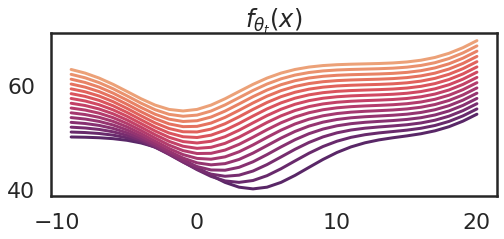
So we are able to see that because the parameter modifications, the kernel additionally modifications. The kernel turns into flatter. An evidence of that is that ultimately we attain a area of parameter area, the place $theta_4$ modifications the quickest.
Why is that this attention-grabbing?
It seems the neural tangent kernel turns into notably helpful when finding out studying dynamics in infinitely large feed-forward neural networks. Why? As a result of on this restrict, two issues occur:
- First: if we initialize $theta_0$ randomly from appropiately chosen distributions, the preliminary NTK of the community $k_{theta_0}$ approaches a deterministic kernel because the width will increase. This implies, that at initialization, $k_{theta_0}$ would not actually rely upon $theta_0$ however is a set kernel impartial of the precise initialization.
- Second: within the infinite restrict the kernel $k_{theta_t}$ stays fixed over time as we optimise $theta_t$. This removes the parameter dependence throughout coaching.
These two details put collectively indicate that gradient descent within the infinitely large and infinitesimally small studying charge restrict may be understood as a reasonably easy algorithm referred to as kernel gradient descent with a set kernel operate that relies upon solely on the structure (variety of layers, activations, and so forth).
These outcomes, taken along with an older identified end result by Neal, (1994), permits us to characterise the likelihood distribution of minima that gradient descent converges to on this infinite restrict as a Gaussian course of. For particulars, see the paper talked about above.
Do not combine your kernels
There are two considerably associated units of outcomes each involving infinitely large neural netwoks and kernel capabilities, so I simply wished to make clear the distinction between them:
- the older, well-known end result by Neal, (1994), later prolonged by others, is that the distribution of $f_theta$ beneath random initialization of $theta$ converges to a Gaussian course of. This Gaussian course of has a kernel or covariance operate which isn’t, normally, the identical because the neural tangent kernel. This outdated end result would not say something about gradient descent, and is usually used to inspire using Gaussian process-based Bayesian strategies.
- the brand new, NTK, result’s that the evolution of $f_{theta_t}$ throughout gradient descent coaching may be described when it comes to a kernel, the neural tangent kernel, and that within the infinite restrict this kernel stays fixed throughout coaching and is deterministic at initialization. Utilizing this end result, it’s potential to point out that in some instances the distribution of $f_{theta_t}$ is a Gaussian course of at each timestep $t$, not simply at initialization. This end result additionally permits us to determine the Gaussian course of which describes the restrict as $t rightarrow infty$. This limiting Gaussian course of nonetheless will not be the identical because the posterior Gaussian course of which Neal and others would calculate on the idea of the primary end result.
So I hope this submit helps a bit by constructing some instinct about what the neural tangent kernel is. In the event you’re , take a look at the easy colab pocket book I used for these illustrations.